A lot has happened since the first part:
Let’s start from the result and work back through the details. I made a bunch of clay tablets, had them fired by Ilse, and put them up for sale on my Etsy store. Here is a photo album to check out:
The reason it took so long to get the second update out is that I wanted to build a proper website with the concept, motivation, tutorials, a gallery, and a webshop. But as a suprpise to no one that’s quite a big project on its own, so I finally decided to write another update on my blog meanwhile.
The first key element to the new proccess is my newfound gcode swiss army knife: vpype. With vpype-gcode turning an SVG or text file into gcode is a one-liner, you just need a config file for your CNC and a few command-line flags.
vpype --config vpype.toml pagesize a5 text --position 1cm 1cm --wrap 12.5cm --size 22pt --hyphenate en --justify "$RANDOM_PAGE_TEXT" linemerge show gwrite --profile cnc random.gcode
But the biggest change was in the preparation of the clay slab itself. I abandoned my failing attempts at making a mold, and followed Ilse’s advice to roll the clay between strips of wood.
Materials needed:
To make a clay tablet you obviously need clay. It is important that the clay contains chamotte, which makes it less likely to explode in the oven. It’s also nice if the chamotte is small to get smooth writing. Clay with 0.2mm chamotte has worked the best for me.
We need a very flat surface, we’re aiming for sub milimeter precision to get consistent writing. Plasterboard is the surface that Ilse recommended, which has worked well for me. (unlike wood which will warp) I cut off roughly square sheets and taped the edges so we can safely move the drying tablets around.
It is very important to work on top of a smooth non-strechy cloth. I use a cut up cotton bedsheet. This allows us to flip the tablet over, inspect it for air bubbles, and prevents it from sticking to the plasterboard and warping while drying.
Now we can get to work. Cut off a piece of clay with a wire cutter, place it on the cloth betweent the wood strips, and use the dough roller to flatten it out. If you’re reusing scraps from a pervious tablet, first knead the clay into a ball, while making sure not to knead any air bubbles.
After rolling it flat we can cut off the excess clay with a knife. I use a folded piece of paper as a reference. Then take the rib and smooth out the surface, making it nice and shiny.
An important step at this point is to slightly lift the fabric, bending the tablet. If there are any air bubbles they will show up as little blisters. Poke them with a knife and flatten the tablet again.
Now cover the tablet with a cloth and flip it over, taking care not to leave fingerprints. Then take the rib and smooth the other side. Then flip it to whichever side looks nicer to become the front.
With my current process I put the entire board with the wet clay tablet right under the CNC. I give it a final roll with the dough roller because clay has a little bit of memory. Then I zero the CNC on the wood strip to get the correct height without leaving a mark. For the CNC bit I actually use a thick needle in a 2mm chuck at 0 RPM, I found that the stationary sharp point produces the finest writing in the wet clay.
A sneak peak at my current experiments is that I’m trying out what happens if you let the clay dry a little bit. Maybe there is a sweet spot where you can CNC it without accumulating or chipping, but I’ve not yet found it. I’m also experimenting with V-carving to be able to engrave more complicated graphics such as mathematical equations. My current goal is to engrave Maxwell equations on a tablet, so that’s a whole new can of worms.
]]>A theremin is an electronic instrument that you play by moving your hands in the air. It uses an analog circuit with two tuned oscillators, one of which is modulated by the antenna impedance which is perturbed by the presence of your body in the near field. The slight frequency differences are fed into a mixer to produce an audible frequency.
A singing bowl is a very old insturment that is usually played by rotating a suede covered mallet around its outside rim. The stick-slip motion of the mallet excites vibration modes of which the nodes are pushed around by the mallet. Some more experimental musicians also play singing bowls by drawing a violin bow across the rim.
A hurdy-gurdy is a string instrument, which uses a hand-cranked wheel with rosin on it rather than a bow. It also has other unique features like drone strings and a keyboard on the neck.
So here is the idea: what if you used a theremin to drive a hurdy-gurdy wheel and use that to play a singing bowl? Magic theremin singing bowl!
For the theremin I built myself a copy of the Thierrymin (using J113 jfets), which I fed into a comparator, stepper motor driver, and stepper motor. From there the only things I had to tweak were a few resistors to add a little hysteresis, and I played around with the microstepping pins to change the speed of the stepper motor. Here is a rough schematic:
That was the easy part. Then I did a bunch of experiments with different types of wheels. I tried rosin, suede, wood, plastic. I tried to spin the wheel on a static bowl, or to spin the bowl against a static baton. It kind of worked, but nothing worked quite the way I wanted it. And then life got rather busy and the project sat dormant for a while. So that’s when I decided to just write a blogpost with my progress and shelve the project. Maybe I’ll get back to it one day, or inspire someone else.
]]>For this page we wanted a simple gauge, so I figured a solution would be an internet search away. But all the examples I found seemed really complicated, with verbose markup, opaque CSS, and sometimes an entire JS library. So I decidede to make my own.
My goals were
The HTML is as simple as it gets, just a div
with custom properties and the textual value.
<div class="gauge" style="--value:0.3; font-size:2rem;">30%</div>
Conceptually, the CSS isn’t very complicated either.
div
border-radius
to make a circleconic-gradiant
to make a pie-chartradial-gradient
to cut out the centertext-align
and line-height
The code CSS makes use of calc
and var
, primarily to adjust the conic-gradient
angle based on a custom property, but also to parameterize the dimensions of the gauge. This means you can override --size
and friends to style the gauge without changing hardcoded values.
.gauge {
--size: 200px;
--cutout: 50%;
--color: red;
--background: white;
width:var(--size);
height:var(--size);
border-radius:calc(var(--size) / 2);
background:
radial-gradient(
var(--background) 0 var(--cutout),
transparent var(--cutout) 100%),
conic-gradient(from -135deg,
var(--color) calc(270deg*var(--value)),
grey calc(270deg*var(--value)) 270deg,
transparent 270deg);
text-align: center;
line-height: var(--size);
}
The JavaScript for changing the gauge value is pretty simple too, given some gauge DOM element el
you can change the gauge value and text content by simply doing
el.style.setProperty("--value", 0.8)
el.innerHTML = "80%"
Below is a codepen to play with the code. I hope it’s useful to someone.
See the Pen Pure CSS gauge by Pepijn de Vos (@pepijndevos) on CodePen.
After a bit of chatting on the Recurse Center Zulip, I came up with the following alternative gradients that provide a 3D effect or that goes from red to orange to green. The 3D one works by adding a transparent black gradient to the radial part. The colourful one works by making a fixed backdrop and a transparent-grey gradient on top that reveals the underlying one.
background:
conic-gradient(from -135deg,
transparent 270deg,
white 270deg),
radial-gradient(
var(--background) 0 var(--cutout),
#0002 calc(var(--cutout)),
#0000 calc(var(--cutout) + 15px),
#0002 calc(var(--cutout) + 30px),
#0000 calc(var(--cutout) + 30px) 100%),
conic-gradient(from -135deg,
var(--color) calc(270deg*var(--value)),
grey calc(270deg*var(--value)) 270deg,
transparent 270deg);
background:
radial-gradient(
var(--background) 0 var(--cutout),
transparent var(--cutout) 100%),
conic-gradient(from -135deg,
transparent calc(270deg*var(--value)),
grey calc(270deg*var(--value)) 270deg,
transparent 270deg),
conic-gradient(from -135deg,
red 0,
orange 135deg,
lime 270deg,
transparent 270deg);
So, how do you build ChatGPT with data compression? What if you compress a large corpus of text to build up the encoding table, then you compress your prompt and append some random data and decompress the random data, and hope it decompresses to something sensible.
It feels vaguely similar to diffusion, but what do I know. Look, this is just a dumb idea, let’s just see what happens ok? Well, here is my progress so far. It’s kind of whack but it’s hilarious to me that it produces something resembling words.
import nltk
import lzma
import random
my_filters = [
{"id": lzma.FILTER_LZMA2, "preset": 9 | lzma.PRESET_EXTREME},
]
lzc = lzma.LZMACompressor(lzma.FORMAT_RAW, filters=my_filters)
corp = nltk.corpus.reuters.raw().encode()
out1 = lzc.compress(corp)
corp = ' '.join(nltk.corpus.brown.words()).encode()
out2 = lzc.compress(corp)
corp = nltk.corpus.gutenberg.raw().encode()
out3 = lzc.compress(corp)
out_end = lzc.flush()
lzd = lzma.LZMADecompressor(lzma.FORMAT_RAW, filters=my_filters)
lzd.decompress(out1)
lzd.decompress(out2)
lzd.decompress(out3)
# mess around to avoid LZMAError: Corrupt input data
lzd.decompress(out_end[:-344])
# insert prompt????
print(lzd.decompress(random.randbytes(50)).decode(errors="ignore"))
Here are a few runs. Note how the start is always , and tri
, usually completing it into some word. Are we doing some primitive accidental “prompting” or just flushing the buffer? Either way, not bad for mere seconds of “training”!
$ python train.py
, and triof billioerse,
But
ht and see th,
Thy smile, in to be happy,
Wmson,
Over tout as aThy smile;t as aThyrged in
ent, foldehe snoion since how long,
my roomr? Is ic books
$ python train.py
, and triompact, sca,
Take deepcky fouy vitaliz bodiehow there i,
Nor drummiwisibly wile of the-ations, dutway?
Yet ld woman'okesmanall whoy slow bekesmanalle me
$ python train.py
, and tri billions of the boftier, faie no acqutory's dazzd haOr that thpages:
(Sometimeseathe ihern, Sounte, fld Turkey n one,
Worlseathe Border Minstrelsy,ine, New-Ene Queen.
'Thelicate l
$ python train.py
, and tri, sleepinlke babes bent,
Abird;
Forhis fair n!
By thea mystic strangehe gifts ofhe body aering
t: I haue a lugs whipageantuperb-fnz
$ python train.py
, and triions of b--n the gra, with
e open the countless buAnd bid theng;
Billi toward you.i ally undya Songs
To f Death, istas of was mar to be UY 9,30
That’s it. That’s the plan. “set in stone” Wikipedia, literally. I know it sounds crazy and I don’t have any illusions about completing the project, but it seems a fun mix of art project and potentially my biggest contribution to the persistence of human kind haha
But how do I go about doing this? I want to automate it as much as possible, but it also has to be super durable and some amount of authentic. Like, if you’re going for pure efficiency and inforation density you’d maybe engrave binary into acrylic, but what’s the fun in that. There are so many remaining options from laser engraving slate to CNC routing clay tablets. Let’s just research and try some?
I started watching a bunch of youtube videos about low fire backyard pottery, where people make pottery on their own improvised coal furnaces and such. Some things I learned:
So I started making my clay tablet by mixing sand into the clay and adding water. Then I used (wet) planks to make the tablet as flat as possible.
Then I copied a wikipedia page into a text file and used hf2gcode to make gcode:
text=$(python - $1 <<END
import unidecode, sys
with open(sys.argv[1]) as f:
print(unidecode.unidecode(f.read()))
END
)
echo "$text" | fold -w 20 | ./src/hf2gcode -s 0.3 -n 12
After letting the clay dry and with my gcode in hand I went to Tkkrlab to try to CNC it. I used bCNC for this. The first try chipped off some bits, so I sprayed some water to make it more soft. But the text was way too small, so I redid the gcode with a bigger font and only the first paragraph of the wikipedia page.
With a bigger font size and regular water spraying I was making good progress, untill the bit started cutting deeper and deeper. Despite my best efforts the tablet wasn’t flat enough, so I had to stop, readjust the CNC, and do some hacky maneuvers to start the job from that point. Success?! Some parts were barely touching, but it’s something!
So I went back home and put it in the oven to dry further. First at below 100, then at 150, and then cranking it all the way up. I guess I was too impatient because it exploded.
So I’m a bit torn, the first two items are probably solvable, and I really love how it looks, but at this font size it can barely fit a paragraph. With a beter process I can maybe reduce it a little bit, in particular the line height is quite excessive, but it’s just not going to fit an entire wikipedia page.
Do I continue pushing this, or do I try something else? I think I might try what laser engraving slate looks like once the laser cutter at Tkkrlab is back in operation.
]]>You see, the sensible thing would be to just run Julia on the EV3 which runs a full Linux, but the modern approach would be to run Julia on the Robot Inventor/Spike Prime Hub, which is an STM32 running a MicroPython firmware.
Here is the game plan. Lacking a MicroJulia implementation and the resources to write a completely custom firmware, we’re going to compile Julia functions into MicroPython extension modules and run them on PyBricks.
This way you can do all your fancy ControlSystems stuff in Julia, compile it to machine code, and then write some Python glue for the sensors and motors.
We’ll basically need to do 3 things
MicroPython has this whole page about how to write native modules in C and compile them into .mpy files. This should be easy!
So I just copied their factorial example, changed ARCH = armv7emsp
, and ran make
to end up with a sweet native .mpy module. Cool now just upload it. Oh. Anyway after some hacks I could use pybricksdev run ble test.py
to upload a tiny test program:
import factorial
print("hello", factorial.factorial(4))
Except it threw ValueError: incompatible .mpy arch
at me no matter what I tried. A little digging later, I found that I needed to enable MICROPY_EMIT_THUMB
. But then I got a weird error in MicroPython, which I hacked around as well.
Then, a small victory: running C code! Now onto Julia.
For the first part I used the amazing AVRCompiler.jl which ties into GPUCompiler.jl which ties into LLVM. Long story short, we can abuse the machinery Julia has for running a static subset of Julia on the GPU for generating machine code for other architectures.
All I did was compile Julia from source1 while adding ARM
to the supported architectures, and changed the target triple in AVRCompiler to the one I found by by copying the CFLAGS from PyBricks and asking LLVM:
clang -print-effective-triple -mthumb -mtune=cortex-m4 -mcpu=cortex-m4 -mfpu=fpv4-sp-d16 -mfloat-abi=hard --target=arm-none-eabi
thumbv7em-none-unknown-eabihf
Once that is in place you can just do
using AVRCompiler
function factorial(x)
if x == 0
return 1
end
return x * factorial(x - 1)
end
obj = AVRCompiler.build_obj(factorial, (Int32,))
write("factorial.o", obj)
So we have a way to run native .mpy modules, and we have a way to compile Julia functions to .o files. Now we just need some glue to link the object file into .mpy and make it accessible from MicroPython.
I basically took the factorial example, ripped out the factorial_helper
and replaced it with extern int julia_factorial(int);
and modified the Makefile to call my Julia script to generate the object file.
# Location of top-level MicroPython directory
MPY_DIR = ../pybricks-micropython/micropython
# Name of module
MOD = factorial
# Source files (.c or .py)
SRC = wrapper.c
SRC_O = factorial.o
# Architecture to build for (x86, x64, armv6m, armv7m, xtensa, xtensawin)
ARCH = armv7emsp
# Include to get the rules for compiling and linking the module
include $(MPY_DIR)/py/dynruntime.mk
# Build .o from .jl source files
%.o: %.jl $(CONFIG_H) Makefile
$(ECHO) "JL $<"
julia --project=. $<
This was all looking really promising until I ran make
and was greeted by
LinkError: factorial.o: undefined symbol: __aeabi_unwind_cpp_pr0
But, yolo, lemme just comment that out in mpy_ld.py
and press on. This symbol appears to be related to exceptions and I don’t really care.
$ pybricksdev run ble test.py
Searching for any hub with Pybricks service...
100%|████████████████████████████| 280/280 [00:00<00:00, 2.15kB/s]
hello 24
At last! Julia code running on the Lego hub! TODO: make cool demo
]]>I started designing the part that clamps the phone, and the tilt mechanism. Everything from building the Lego set to making the tripod was basically an excuse to use these linear screw cylinders in my builds. The clamp is made of these rounded pieces to hold the phone, with a 5.5 axle with stop sandwiched between cross blocks to provide a stiff adjustable size. From there I just tried to find the most compact and straightforward way to attach the linear screw cylinder.
Next I wanted to be able to raise and lower the phone. At first I wanted to use scisor lift mechanism, but quickly realised it’d be too complicated. Instead I went for a car jack mechanism. The set comes with just the right amount of gears and liftarms. The only downside is that the gears have to be offset half a tooth so it’s not exactly straight. It also wasn’t very stable at first, but after adding the center bar, it’s acceptable. Just give it a bit of help when tryig to raise the jack while a phone is inserted.
Then it was just a matter of connecting them together with the turntable. Here it is in the lowest and highest position.
To use my phone as a camera, I use DroidCam OBS
]]>The TL;DR is the only thing that actually sucks about your router is the WiFi coverage. Use the wired network and/or put some extra access points in strategic locations.
Literally any router can do 1000Mbps, which is enough for multiple 4K video streams. But chances are the router is stuffed away somewhere in a corner of the hallway. Of course WiFi on the other end of the house is going to suck. The solution is simple: place some extra access points in strategic locations throughout the house.
But let’s go back to the beginning. Since we’re both working from home, I had just upgraded our internet to the fastest fiber available in the area, 1000Mbps, and in the progress discovered I can change my WiFi password from the website of my ISP, meaning my ISP has remote access to my router. Not cool. And if I was going to revise the setup, I had a few other ideas
And from there it went a bit like this. And like my Linux journey, there came a point where I just want stuff to work reliably rather than always having the new hotness.
The idea was that if I used a repurposed thin client combined with a PoE switch, that I could plug in an SFP+ card for a fiber transciever and an easy 10GbE upgrade path, transfer the Raspberry Pi’s duties to the thin client, and power the access points from the PoE switch.
The easy part was picking access points. I just selected some TP-Link Omada WiFi 6 access points. For the switch I initially selected a fairly simple PoE switch, but then realised I’d need a managed switch for my IoT VLAN, and then I figured why not an Omada managed switch so I could control everything from one place. But, foreshadowing, the Omada managed switch wasn’t that much cheaper than a full Omada PoE router with built-in controller.
At this point I was under the impression my fiber was GPON and not compatible with the available SFP trancievers, so 10GbE SFP+ cards would be for another day. Finding a network card was actually the hardest, because many of the older and cheaper NICs have a higher TDP than would be wise to put into such a small PC, and often use brands that don’t have great support in DPDK or FreeBSD. Eventually I found a two port Intel NIC.
For the thin client, I spent a bunch of time searching for ones that have PCIe slots, such as the HP t620 PLUS, Fujitsu FUTRO S920, and the final choice, Lenovo ThinkCentre M720 Tiny. The Fujitsu is a much cheaper option, but I had 10GbE in mind and also wanted to use it as a home server, so opted for a bit more powerful machine. Serve The Home was a great resource in this journey.
Here is where the setbacks started:
At this point I was having my doubts, but sunken cost fallacy kept me going. I also just like to play with tech toys. So once the riser arrived I proceeded to set it up as a router.
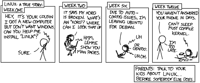
At first I was planning to go with OpnSense, but then a friend told me that kernel mode routing is so slow, and all the cool kids use DPDK these days, so why not use DANOS or VPP? Who needs a web GUI anyway. [Week six]
So I installed Ubuntu Server and VPP, and then moved on to their VPP as a home gateway page.
What that page neglects to mention is how to get your kernel to give up the normal network driver so that DPDK can use it.
It turns out that if you apt install dpdk
it installs a service that automatically does this for you after you obtain the IDs of the NIC with lspci
and add them to /etc/dpdk/interfaces
:
pci 0000:01:00.0 vfio-pci
pci 0000:01:00.1 vfio-pci
Then I decided I wanted to use dnsmasq as both the DNS and DHCP server, which has the benefit that you can access your devices by their hostname. I settled on the following /etc/dnsmasq.conf
which binds to the VPP bridge interface, ignores, resolv.conf
, uses Google DNS, a .lan domain, adds DHCP hosts to the DNS, sets the gateway to VPP, and the DHCP server to itself.
interface=lstack
no-resolv
server=8.8.8.8
server=8.8.4.4
local=/lan/
domain=lan
expand-hosts
# Set default gateway
dhcp-option=3,192.168.5.1
# Set DNS servers to announce
dhcp-option=6,0.0.0.0
When I was setting up VPP, the configuration files they provided were essentially broken, resulting in a long struggle to get NAT working. The documentation has since been updated, which is potentially a better reference than below config.
/etc/vpp/startup.conf
:
unix {
nodaemon
log /var/log/vpp/vpp.log
full-coredump
cli-listen /run/vpp/cli.sock
startup-config /setup.gate
gid vpp
poll-sleep-usec 100
}
api-trace {
on
}
api-segment {
gid vpp
}
socksvr {
default
}
dpdk {
dev 0000:01:00.0
dev 0000:01:00.1
}
plugins {
plugin default { disable }
plugin dpdk_plugin.so { enable }
plugin nat_plugin.so { enable }
plugin dhcp_plugin.so { enable }
plugin ping_plugin.so { enable }
}
setup.gate
:
define HOSTNAME vpp1
define TRUNKHW GigabitEthernet1/0/0
define TRUNK GigabitEthernet1/0/0.300
define VLAN 300
comment { Specific MAC address yields a constant IP address }
define TRUNK_MACADDR 90:e2:ba:47:df:ec
define BVI_MACADDR 90:e2:ba:47:df:ed
comment { inside subnet 192.168.<inside_subnet>.0/24 }
define INSIDE_SUBNET 5
define INSIDE_PORT1 GigabitEthernet1/0/1
exec /setup.tmpl
setup.tmpl
:
show macro
set int mac address $(TRUNKHW) $(TRUNK_MACADDR)
set int state $(TRUNKHW) up
create sub-interfaces $(TRUNKHW) $(VLAN)
set int state $(TRUNK) up
set dhcp client intfc $(TRUNK) hostname $(HOSTNAME)
bvi create instance 0
set int mac address bvi0 $(BVI_MACADDR)
set int l2 bridge bvi0 1 bvi
set int ip address bvi0 192.168.$(INSIDE_SUBNET).1/24
set int state bvi0 up
set int l2 bridge $(INSIDE_PORT1) 1
set int state $(INSIDE_PORT1) up
comment { dhcp server and host-stack access }
create tap host-if-name lstack host-ip4-addr 192.168.$(INSIDE_SUBNET).2/24 host-ip4-gw 192.168.$(INSIDE_SUBNET).1
set int l2 bridge tap0 1
set int state tap0 up
nat44 forwarding enable
nat44 plugin enable sessions 63000
nat44 add interface address $(TRUNK)
set interface nat44 in bvi0 out $(TRUNK)
Note that without the poll-sleep-usec
command, the CPU will be at 100% all the time, which is not very power efficient. But taking a high performance user space dataplane for low latency and then inserting a delay seems kinda pointless doensn’t it? But even with the delay, it was plenty fast in my testing, saturating the uplink without any obvious extra latency.
One significant difference in my config is that my ISP requires a VLAN of 300 on the WAN port, which was another struggle. The solution is that you have to set up a sub-interface like GigabitEthernet1/0/0.300
which will add the VLAN tag on outbound traffic and strip it on inbound trafffic. You then have to use this subinterface for all further setup.
While initially I tested VPP as a secondary router behind the ISP router, the VLAN struggle had to happen while my girfriend was without internet, another moment of realisation: I am now managing a sever exposed to the public internet, and if there is an issue we’re without internet access. Do I want that kind of responsibility for fun?
Is there any way I can justify this project? Time to do some testing. 
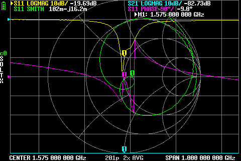
First I ran speedtest.net on the ISP router and the VPP router, and the results are pretty much indistinguishable. Around 8ms latency and 930Mbps up and down. But then my friend said the real test is packets per second, not just megabits, so I went to iperf3 and basically failed to run any test that would show a significant difference. That is, UDP tests with small packets would just kinda hang, and TCP tests would report similar numbers to Speedtest.
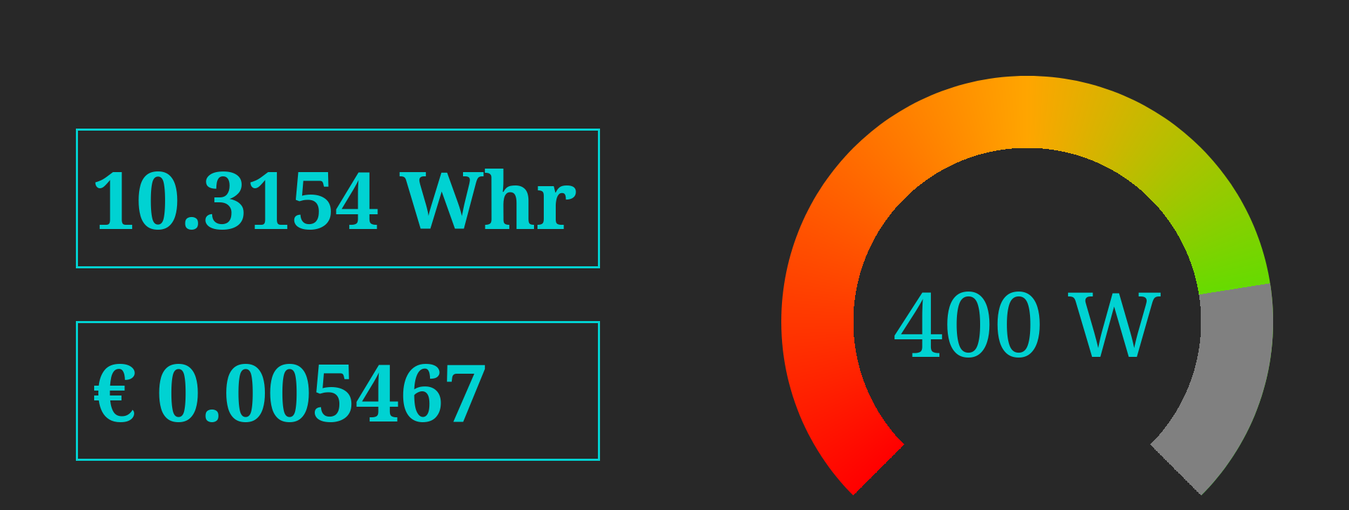
The other metric I looked at is wall power. Turns out the Raspi uses around 2W and the ISP router 18W, while the VPP router uses 20W. I slightly rounded the numbers for effect, but it’s not an obvious win. And that’s without the access point and switch this setup would need.
So in the end it’s not faster or more efficient, and a hecking lot more maintenance. Assuming the new fan would be sufficiently silent. And then my girlfriend said her Skype calls kept dropping upstairs, which is when I decided to quit messing around and buy a setup that just works.
At this point I had kind of dismissed 10GbE as uneccessery, expensive, and power hungry. It also occured to me that if routers were actually bad, router companies would be put out of business by kids selling preconfigured pfSense thin clients. So I asked the owner of Routershop.nl for advice, and just bought whatever he recommended.
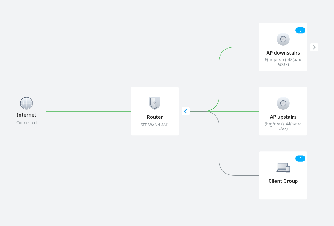
The router is a fanless 3-in-1 Gigabit router, PoE switch, and Omada controller. It has 12 ports, of which 2 SFP cages, and a generous 110W PoE budget. The access point just a random Gigabit Wifi 6 device. More than sufficient for my needs for the forseeable future.
Around this time I also found a thread on my ISP’s forum where I learned that my fiber is actually AON, and which type of SFP module I need. I confirmed this information with customer support and the Routershop guy. The module he sold me slots right into the router and worked on the first try. Bye media converter!
I guess I’ll just keep the Raspberry Pi around, and equip it with a PoE+ hat for fun.
Getting to the same point as the VPP router was a breeze: The setup wizard detected the access points and configured the main WiFi network. Then I just had to go to settings, wired network, internet, select the WAN port, and then under advanced settings put the Internet VLAN to 300. I first did this with the media converter, and once confirmed working, did a speed test, and switched the fiber from the media converter to the SFP module. Once again the test results were indistinguishable. Et voila, new network.
For science, I powered on the old router, to compare the reception upstairs in the furthest corner of the house. With my laptop on my lap I could not even see the old 5GHz network, but putting it down I captured the following image, with in purple the old WiFi, and red and gree respectively the downstairs and upstairs access points. Not only is it obvious why WiFi was so bad upstairs, it also shows how much better the dedicated access points are. The new downstairs AP comes through almost 20dB stronger than the old router. We could probably have made do with just the new downstairs AP.
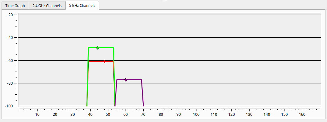
While I’ve repeatedly found that any of the 3 routers can saturate a 1000Mbps link, WiFi is a different story. The new AP is actually 200Mbps faster than the old ISP router, while sitting about 3m away from each. Note that my laptop doesn’t have WiFi 6 so this is probably leaving speed on the table. But of course the wired network remains faster and more reliable.
The one feature missing from the Omada setup compared to VPP is that it doesn’t run a DNS server, so you can’t access devices by their hostname. But if I’m running the Raspberry Pi anyway I could run dnsmasq there if I wanted to. Or even Pihole while I’m at it.
Now that I have this easy to manage network, it’s time to tick off the last item on my wishlist: put all the IoT stuff on its own VLAN. I found this video quite helpful, even though my setup is a bit different.
I actually have two types of IoT devices. Cloud based ones that I begrudgingly allow internet acccess so that their app works. And local ones that talk to Home Assistant and have no business connecting to the internet.
The cloud one is simple, make a new WiFi network, and tick “guest mode”. This prevents it from connecting to any other device on the network. For the Home Assistant devices, I made a new LAN (purpose: interface, apparently), and gave it a nice VLAN ID and DHCP setup. Then I created another WiFi network, no guest mode, same VLAN ID.
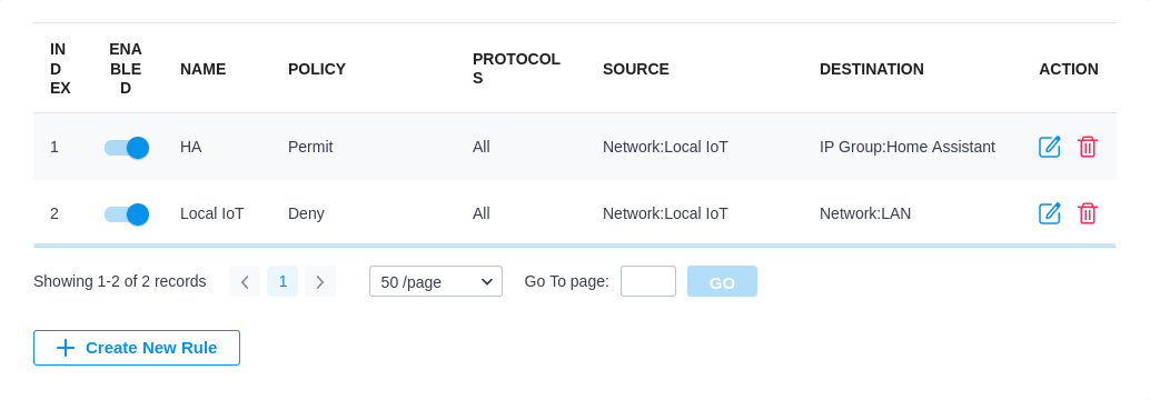
Home Assistant itself actually runs on the main LAN so it can access the internet and it’s easy to target all the IoT devices. First I added a gateway rule from LAN to WAN that denies the IoT network to the IP group Any_IP. Then I added two EAP rules, one that allows the Iot network to a new IP group with just Home Assistant in it (which I assigned a static IP), and then a deny rule that denies the IoT network to the default LAN network.
You can make your own router, but there isn’t really a good reason to in my opinion. I could not find any measureable advantage. You can do it if you are looking for a new hobby, or if you have really specific requirements.
Even if you’re on a budget, the 50 Euro version of this build is just a single WiFi 5 access point, which would probably get you 90% of the way. You could repurpose an old PC if you don’t care about the energy bill and care a lot about your ISP not having remote access to your router I suppose. But with current energy prices the venn diagram of people who can’t afford a new router and care about their energy bill is almost a cricle.
I’m quite happy with the new setup, but in particular the access points are just much better than what’s built into the ISP router.
]]>I consulted several books and papers. A regular patch antenna is a pretty common and simple thing, but GPS is a circularly polarized signal, and that part is a bit more obscure.
To start simple I decided to make a regular patch antenna first and then try to modify it for circular polarization. So I took some equations from the Belanis book and arrived at the following code to calculate the dimensions for a rectangular patch antenna for the L1 GPS frequency of 1574MHz:
from scipy.constants import c, mu_0, epsilon_0
import math
f0 = 1574e6
eps_r = 4.5
h = 1.6e-3
# CP uses this as initial guess for L too
W = c/(2*f0)*math.sqrt(2/(eps_r+1))
print("W:", W*1e3, "mm")
eps_eff = (eps_r+1)/2 + (eps_r-1)/2*(1+12*h/W)**-0.5
print("eps_eff:", eps_eff)
DL=h*0.142*((eps_eff+0.3)*(W/h+0.264))/((eps_eff-0.258)*(W/h+0.8))
print("DL:", DL*1e3, "mm")
L = 1/(2*f0*math.sqrt(eps_eff*mu_0*epsilon_0))-2*DL
print("L:", L*1e3, "mm")
That it pretty much the extent of analysis I did. For the feedline I used the KiCAD PCB calculator to calculate the width of a 50Ω transmission line. To fine-tune everything I just did a lot of parameter sweeps in the simulator.
As far as designing the CP antenna goes, none of the books IMO strike a good balance of giving useful and understandable theory about CP. They kind of hand-wave about disturbances and throw some integrals at you. So in the end I just went with the truncated corner design and did some sweeps on how much to chop off.
At first I tried to simulate the antenna with OpenEMS, based on modifying their simple patch antenna tutorial. But I got really weird results and kind of gave up on that idea. I had seen Andrew Zonenberg do a lot of EM simulations in Sonnet, and they were kind enough to provide me with a trial license for this project, as well as amazing support. I really can’t recommend them enough. As Andrew says: OpenEMS might be good in the future, but right now if you value your time, Sonnet is the way to go.
My analysis suggested a patch size of around 45mm, so I tried to set up a sweep in Sonnet, but was having issues where different widths would give exactly the same results. I’m just going to quote the entire email I received from their support, who are total experts in their domain:
The reason why you are observing stepped behavior in your parameter sweep responses is because the variable step is smaller than the cell size and the metal is off grid. The variable L is swept from 44 to 46 mm, with a step of 0.1 mm: 
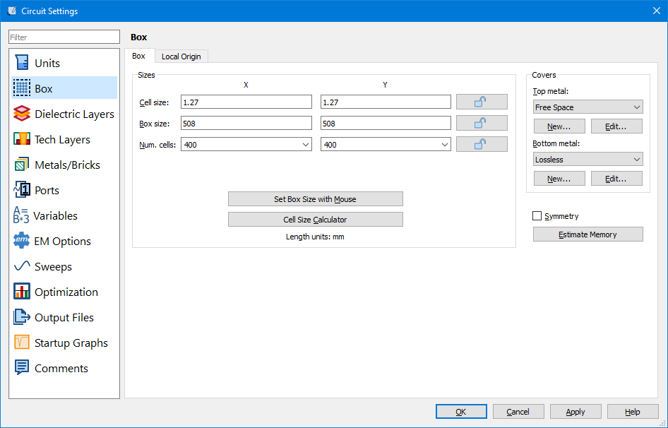
The cell size is 1.27 x 1.27 mm: 
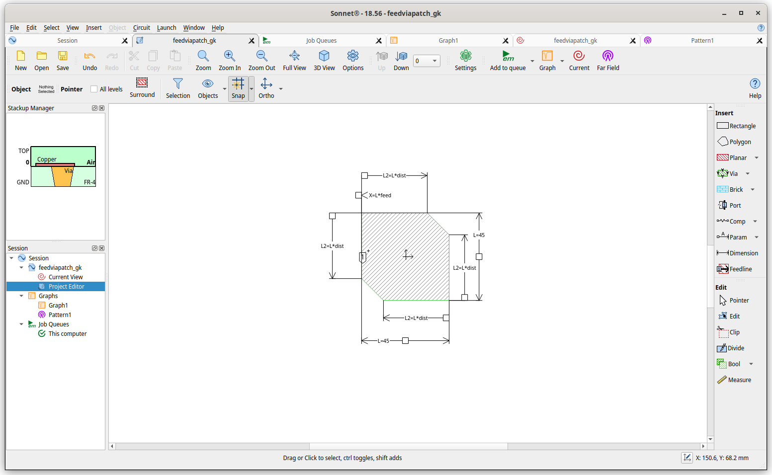
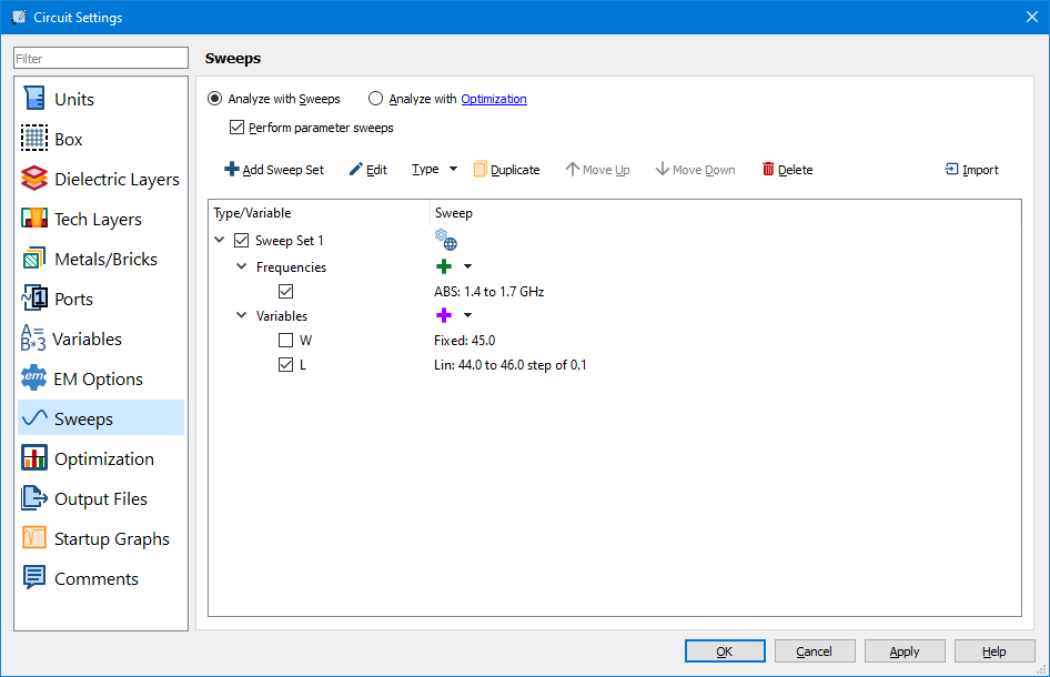
Below is a screenshot of the geometry with the dimension parameters displayed: 
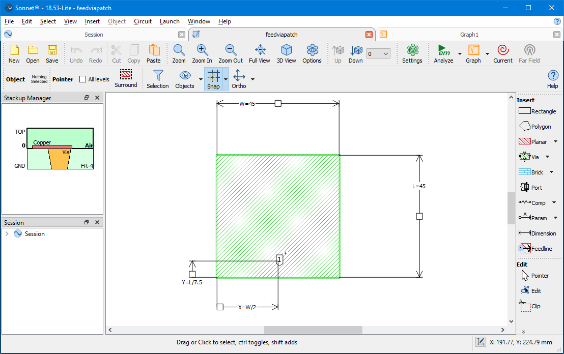
The Sonnet EM solver analyzes the metal as it is snapped to the grid. This means the following:
- When L is 44 mm, the metal snapped to the grid is 44.45 mm (35 cells).
- When L is 45 mm, the metal snapped to the grid is 44.45 mm (35 cells).
- When L is 46 mm, the metal snapped to the grid is 45.72 mm (36 cells).
The dependent parameter Y equals L/7.5 mm.
- When L is 44 mm, Y = 5.866 mm. The snapped dimension would be 6.35 mm (5 cells).
- When L is 45 mm, Y = 6.0 mm. The snapped dimension would be 6.35 mm (5 cells).
- When L is 46 mm, Y = 6.133 mm. The snapped dimension would be 6.35 mm (5 cells).
With the specified parameter sweep of L of 44 to 46 mm, step of 0.1 mm, effectively the L dimension is 6.35 mm in all combinations. The key then is to work with a smaller cell size, to resolve the small dimensional changes. A smaller cell size will increase the memory requirement and analysis time, so there is a tradeoff. In the attached “feedviapatch_gk” model variation, I made a number of modifications:
- Cell Size – Reduced cell size from 1.27 x 1.27 mm to 0.2 x 0.2 mm. This will resolve smaller dimension changes and match the patch dimensions better, which are whole numbers 45 x 45 mm
- Via Port- The via size for the Via Port was 1.27 x 1.27 mm. I snapped this via to the new grid, reducing it to 1.2 x 1.2 mm. This should have minimal impact on the response.
- Box Size - Wavelength with Er=1, at 1.575 GHz is 190 mm. For antenna models, we recommend approximately 2 wavelengths or more clear area around the antenna. Specified a box size of 800 x 800 um, which is a reasonable size. With a relatively large box size and relatively small cell size, this will lead to a large number of cells. In this model it is 4000 x 4000 number of cells, which is reasonable. As the number of cells reaches 20000 or more, the analysis time will increase substantially.
- Upper air layer thickness – With an antenna model, with the box bottom cover used as a lower groundplane, the upper air layer thickness should be approximately 0.5 wavelength. Specified a value of 95 mm.
- Patch position and orientation – Centered the patch and rotated it 90 degrees clockwise
- Symmetry – Enabled symmetry. With the centered patch and new orientation, symmetry can be used to substantially reduce the memory requirement and analysis time.
- Via Port position variable – Deleted the existing X and Y dimension parameters. Redefined a new X parameter. A new Y dimension parameter was not required as the Via Port remains centered.
- Parameter sweep - Changed parameter sweep of L to 44 to 46 um, step 1 mm. All of the L values will be resolved and fall on the grid. The X values will be 5.866, 6, and 6.133 mm. Due to the 0.2 x 0.2 mm grid, these will be snapped to 5.8, 6, and 6.2 mm.
Below is a dB[S11] plot comparing the response at L values of 44, 45, and 46 mm: For finer resolution, you could use a 0.1 x 0.1 mm cell size, but this will come at the expense of additional memory and analysis time. The change in the X variable value will drive the cell size. For example a 1 mm change in L, results in a 1/7.5 = 0.133 mm change in X.
For this model, the total analysis time on my desktop machine was 5 minutes, 37 seconds. The reported memory requirement was only 2 MB, because the Lite EM solver only counts one portion of the analysis. You can see the actual memory requirement in the logfile, which was 146 MB.
The attached model is a packed project archive (zon extension) with data. You can open it as you would a project file (son extension). Since it already includes data, you do not need to reanalyze and can plot the S-parameter and current density data.
Wow I did a learn. Amazing. After that I could easily run some sweeps and find an antenna size suitable for GPS reception. From here things happened kind of in parallel, but for the sake of the story let’s move on to simulating the CP antenna.
I had two more minor problems with this antenna. First is that it’s no longer symmetrical so I should turn off that setting again. The other is that circular polarization requires far-field analysis, and far-field analysis requires a full EM solve at the desired frequency. When you just do a normal sweep Sonnet tries to be smart and interpolate a bunch of things, so if you want to compare data from different parameters, you actually need to tell it to do a full EM solve at that frequency by adding a linear sweep and/or a single frequency.
Then you can set up and parameterize a truncated patch and do some sweeps:
Here is the S11 of my final antenna and some sweeps of the axial ratio of the far field.
After the simulations it was finally time to make some antennas. I decided the best way to prototype these things was to use the CNC at Tkkrlab to mill a double sided PCB blank into an antenna and solder some SMA connectors to it. First I drew the antenna in KiCAD using SMD pads as the patch, there is even an option to make chamfered pads. I also added a stripline to callibrate the width.
Then I exported the PCB design to Gerber, loaded it into FlatCAM to convert it to a toolpath, and used bCNC to execute it. The process is a bit unintuitive and requires some experimentation, but nothing too crazy. I was able to just show up to Tkkrlab with my gerber files, create toolpaths, put on PPE, and watch my antenna being made. I used a 3mm flat bit to clear all the metal, and then a pointy bit to route the edges for exact dimensions and to get the SMA pads cut.
For testing the impedance of the antenna as well as the S11 I got myselve a LiteVNA. For the rectangular patch, I cut slots at the feedline to reduce the impedance, and for the truncated patch I was worried I’d have to construct some RF magic like a quarter wave transformer or hybrid but for some reason the impedance was actually kinda alright. Here is what the readout of the truncated andenna looks like:
If you’ll look back at the simulated S11 you’ll see it’s pretty close! Exciting stuff.
So of course the next step is to actually receive GPS signals with it. But how? I went for a two-pronged approach. I ordered an RTL-SDR, which I read can do GPS, and I ordered a PCB with my patch antenna and an u-blox MAX-M10S.
I never got to the SDR part, because the u-blox actually worked!!! It took a bit of fiddling to figure out how the I2C interface worked, but what you see in this picture is my GPS SAO PCB plugged into a MCH badge spewing NMEA messages to my laptop. I blurred the details, but it actually saw satelites and found my location!
All the stuff is on github although it’s more about the process than drawing a 45mm pad ;)
]]>So we set out to add some mushrooms to my computer. One super cool thing my friend added is to use glow in the dark powder instead of paint, and to use UV LEDs. This way your mushrooms are glow in the dark, and keep glowing even if you turn off your PC. Magical!
I hooked them up with 600Ω resistors to the 12V RGB port on my motherboard. This way you can make them fade in and out and do other fun things. A challenge is that there is no control software for Linux, so you have to just set it up on Windows and it seems like the default patterns keep working after you boot into Linux.
]]>