Wishful Coding

So quantization is kinda bad lossy compression right? JPEG is good lossy compression. This may sound stupid, and maybe it is, but hear me out.

I’ve read that LLM performance is usually constrained by memory bandwidth, and for us plebs also by memory size, and there is a precedent in for example ZFS compression which has shown to increase disk performance because you’re IO constrained rather than compute constrained. So it might be beneficial to decompress LLM parameters on the fly, and if you’re doing that you might want to use a good lossy compression algorithm instead of blunt quantization. It is said that compression is equivalent to general intelligence, so in that sense lossy compression would be expected to reduce intelligence, so you’d want to get a good compression ratio with minimal loss.

The way JPEG works is basically

• break down the pixels in chunks - after decompression chunk boundaries are visible as JPEG artifacts.
• Discrete Cosine Transform them - lossless transformation in the family of Fourier transforms
• quantize them - data loss happens here, creating longer runs
• Run Length Encode them - compression happens here

RLE is a lossless compression technique, which gets turbocharged by discarding some data to create longer runs. In the case of image data, the DCT concentrates most information in the low frequencies so you can quantize high frequencies with minor loss in image quality. Now, I don’t expect LLM parameters to be “smooth” like image data, so naive JPEG compression of LLM weights is not likely to be effective.

BUT!

You can reorder the columns and rows of a matrix without affecting the result. It’s like \(a+b+c=d \rightarrow c+b+a=d\). So you could reorder your rows and columns to maximize clustering of similar values. Not sure how you’d do this, maybe just sort by vector sum, or some genetic algorithm, or other cleverness.

So my proposed LLM compression would work like this

• reorder the matrices to improve value clustering
• break down the values in chunks
• DCT them
• quantize them
• RLE them

And then inference would

• RLE expand a chunk
• inverse DCT it
• perform the multiplications

So the compressed data would exist in VRAM and be decompressed on the fly chunk by chunk to perform a matrix vector product. It’d take more compute, 11 multiplications to be precise, but if you’re memory constrained it could be worth it.

I guess the real question is if you can obtain any useful clustering in LLM data. In a sense the parameters are already compressed(=intelligence), but there is no information in their order, so reordering and transforming parameters could improve RLE compression without incurring extra quantization loss.

I got a litlte bit nerd sniped by the following video and decided to implement game of life in clojure.core.logic, because any logic program can be evaluated forwards and backwards.

Without further ado here is my implementation:

(ns pepijndevos.lifeclj
  (:refer-clojure :exclude [==])
  (:use clojure.core.logic)
  (:gen-class))

;; A helper to get the neighbouring cells.
;; Clips to zero.
(defn get-neighbours [rows x y]
  (for [dx (range -1 2)
        dy (range -1 2)
        :when (not (= dx dy 0))]
    (get-in rows [(+ x dx) (+ y dy)] 0)))

;; Produces binary vectors of a certain number of bits.
;; This is used to generate all neighbour combinations.
(defn bitrange [n]
  (sort-by #(apply + %)
           (for [i (range (bit-shift-left 1 n))]
             (vec (map #(bit-and 1 (bit-shift-right i %)) (range n))))))

;; Encode the game of life rules as a 256 element conde.
;; Depending on the number of ones in a vector,
;; the corresponding rule is generated
;; that equates the pattern to the neigbours
;; and the appropriate next state.
;;
;; This can be asked simply what the next state is for
;; given neighbours and current state.
;; OR you could drive it backwards any way you like.
(defn lifegoals [neigh self next]
  (or*
   (for [adj (bitrange 8)
         :let [n (apply + adj)]]
     (cond
       (or (< n 2) (> n 3)) (all (== next 0) (== neigh adj))
       (= n 3)              (all (== next 1) (== neigh adj))
       :else             (all (== next self) (== neigh adj))))))

;; Relate two grids to each other according to the above rules.
;; Applies lifegoals to every cell and its neighbours.
;; in the forwards direction executes one life step,
;; in the backwards direction generates grids
;; that would produce the next step.
(defn stepo [size vars next]
  (let [rows (->> vars (partition size) (map vec) (into []))
        neig (for [x (range size)
                   y (range size)]
               (get-neighbours rows x y))]
    (everyg #(apply lifegoals %) (map vector neig vars next))))

;; Make a grid of unbound variables.
(defn grid [size] (repeatedly (* size size) lvar))

;; Simply execute a life step on the state.
(defn fwdlife [size state]
  (let [vars (grid size)
        next (grid size)]
    (run 1 [q]
         (== q next)
         (== vars state)
         (stepo size vars next))))

;; Produce three backward steps on state.
(defn revlife [size state]
  (let [start (grid size)
        s1 (grid size)
        s2 (grid size)
        end (grid size)]
    (run 1 [q]
          (== q [start s1 s2 end])
          (== end state)
          (stepo size s2 end)
          (stepo size s1 s2)
          (stepo size start s1)
         )))

;; Nicely print the board.
(defn printlife [size grids]
  (doseq [g grids]
    (doseq [row (->> g (partition size) (map vec) (into []))]
      (doseq [t row]
        (print t ""))
      (print "\n"))
    (print "\n")))

;; Test with a glider.
(defn -main [& args]
  (->> [0 0 0 0 0 0
        0 0 0 0 0 0
        0 0 0 1 1 0
        0 0 1 1 0 0
        0 0 0 0 1 0
        0 0 0 0 0 0]
       (revlife 6)
       first
       (printlife 6)))

output:

$ clj -Mrun
1 0 1 0 1 1 
1 0 0 0 0 1 
0 0 1 0 0 0 
0 0 0 0 0 1 
1 0 1 1 0 0 
1 0 1 1 1 1 

0 1 0 0 1 1 
0 0 0 1 1 1 
0 0 0 0 0 0 
0 1 1 1 0 0 
0 0 1 0 0 1 
0 0 1 0 1 0 

0 0 0 1 0 1 
0 0 0 1 0 1 
0 0 0 0 0 0 
0 1 1 1 0 0 
0 0 0 0 1 0 
0 0 0 1 0 0 

0 0 0 0 0 0 
0 0 0 0 0 0 
0 0 0 1 1 0 
0 0 1 1 0 0 
0 0 0 0 1 0 
0 0 0 0 0 0

Sadly, this is nowhere near fast enough to solve the play button problem.

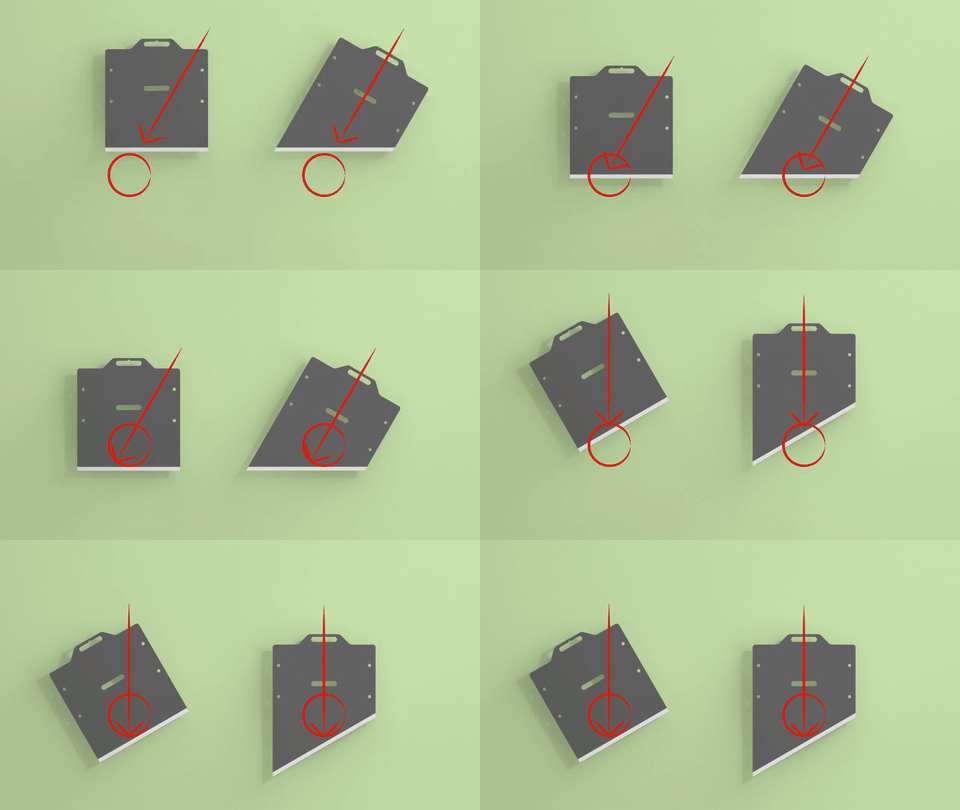
This is a theoretical counterpart to an experimental collaboration between KnowArt and Proper Printing to see if a diagonal guillotine blade cuts better than a horizontal one.

A raised guillotine blade has a certain potential energy which is transferred to the contact point between the blade and the neck. So let’s assume a frictionless spherical cow, I mean neck, and calculate the contact point, force, and energy as a function of the angle of the blade.

The equation of a circle is given by \(x^2-y^2=r^2\), so a horizontal blade intersecting the circle of radius \(r\) at height \(y\) intersects the circle at \(x=\pm\sqrt{r^2-y^2}\). The length of the cut is therefore \(L(y)=2\sqrt{r^2-y^2}\).

For a diagonal blade, we can rotate the reference frame to be aligned to the blade, such that the knife has a horizontal component of \(y\sin(\theta)\) and a vertical component of \(y\cos(\theta)\), creating a contact patch of \(L(y\cos(\theta))=2\sqrt{r^2-y^2\cos^2(\theta)}\).

So now we can express the force from the contact area in terms of some constant \(k\) as \(F(y)=kL(y)\) perpendicular to the blade edge, resulting in a vertial and horizontal component:

This means that an angled blade creates “leverage” where less force but a longer travel is required. To be precise, the travel is given by \(\frac{2r}{\cos(\theta)}\).

To compute the total energy required for a cut, assuming the dominant force scales with the length of the contact patch, is the integral of the force over the vertical travel component.

Now we can simplify by substituting \(u=y\cos(\theta)\), \(dy=\frac{du}{\cos(\theta)}\) and adjust the integration bounds accordingly, cancelling all \(\theta\) terms!

So just as much vertical energy is required to cut through the circle no matter the angle, but we’re also excerting a horizontal force. If the guillotine blade is running on math bearings this is of no concern, but for a wooden sled there is a (Coulomb) friction of \(F_c=\mu F_x\) giving

But what about the pointy blade? I’m not glad you asked because the math is more messy. We can consider one half of the pointy blade at a rotated reference frame. So we get the same \(L\) as before, but now the blade stops at the tangent line of the blade angle, as follows. But then once the point of the blade exits the circle it becomes two flat sections, forming a piecewise function.

For the first part we have half of a flat blade length \(L\), the uncut section \(M\), and the pointy blade section \(N\)

Giving us

For the total work, we already know the square root terms are independent of the angle. And since the sum of the integral is the same as the integral of the sum, we only need to concern ourselves with the \(\sin(\theta)h\) term.

So all our blades take the same amount of work to cut through an uniform saussage, with the diagonal blades being worse due to friction. The brachistochrone blade is left as an exercise to the reader.

But there is more to cutting than uniform math saussages. KnowArt indeed found that the diagonal blade seemed to perform worse than the flat blade due to friction. But the pointy blade performed better. The most likely explanation for this is that a horizontal slicing motion is beneficial for cutting. This makes intuitive sense to anyone who’s done some cooking, and was also explained to me by a medical doctor relative as the difference between a sword and a sabre.

But the story goes that the real reason the blade is diagonal is that the king suggested it might help with people with fat necks. Ironically his own fat neck ended on the block some time later.